机器学习基石笔记第一章：感知机算法（PLA）

机器学习的基本框架
一个简单的学习模型：感知机
- 无噪音数据
- 针对有噪音数据：Pocket算法

机器学习的基本框架

Unknown target function $f$: $\mathcal{X} \to \mathcal{Y}$
Trainning examples $(\mathbf{x}_1, y_1), (\mathbf{x}_2, y_2), \cdots, (\mathbf{x}_N, y_N)$
Hypothesis set $\mathcal{H}$
Learning Algorithm $\mathcal{A}$
Final hypothesis $g$

学习(learning)是利用现有的资料(trainning examples)，通过一些方法步骤(Algorithm)，从我们事先认为有可能的一堆函数(hypothesis set)中找到一个和目标函数$f$“最像”的函数$g$。

下面的五个例子来自于Learning From Data书中的Exercise1.1，让我们来更具体的了解下机器学习的各个组成部分吧！

Example 1: Medical diagnosis A patient walks in with a medical history and some symptoms, and you want to identify the problem.

输入空间	输出空间	目标函数
病人过往病史和当前症状	是否患病	判别函数

Example 2: Handwritten digit recognition(for example postal zip code recognition for mail sorting).

输入空间	输出空间	目标函数
手写数字图片	0~9	判别函数

Example 3: Determine if an email is spam or not.

输入空间	输出空间	目标函数
邮件内容	是否为垃圾邮件	判断函数

Example 4: Predicting how an electric load varies with price, temperature, and day of the week.

输入空间	输出空间	目标函数
电价、气温和日期	电量负载	预测函数

Example 5: A problem of interest to you for which there is no analytic solution, but you have data from which to construct an empirical solution.

输入空间	输出空间	目标函数
现有数据	问题的结果	经验解决方案

一个简单的学习模型：感知机

感知机(Perceptron)是最简单的二元线性分类器，如果我们的数据是线性可分的(Linearly separable)，那它一定能在有限步之内找到一条”线”把正负样本分开。感知机学习算法(Perceptron Learning Algorithm)的主要精神是“知错能改”：在每一轮迭代中，它会先找到一个错分点，然后对其进行修正，尽可能弥补之前的过错。当然，由于一次只关心这一个点，可能这次更新后其他点的情况变得糟糕了，但是感知机会说：“别担心，我们接下来会改的！”

无噪音数据

import numpy as np
import matplotlib.pyplot as plt

首先，我们假设目标函数 $f$ 为线性函数 $f(\mathbf{x})=\mathbf{w}^T\mathbf{x}$ ，其中 $\mathbf{w}=(-1, 2, -1)^T$ , $\mathbf{x}=(x_0, x_1, x_2)^T.$

# Target function: -1 + 2x1 - x2
w = np.array([-1, 2, -1])

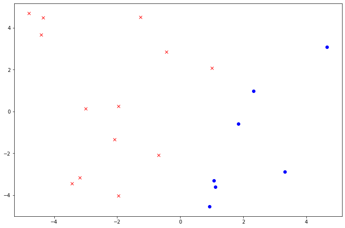
接着，从 $d$ 维立方体 $[-5, 5]^d$ 中随机生成样本大小为$N$的模拟数据，这里假设 $d=2$，$N=20$. 利用目标函数将数据打上标签（+1或-1)，也就是说数据本身是线性可分的，因此PLA一定会收敛。

N, d = 20, 2 # Sample size, number of features

def generateXY(N, d, w):
    """
    Generate a random sample X of size N from a d-dimensional uniform distribution: [-5, 5]^d.
    Label each point by the target linear function described by weight vector w.
    
    Args:
        N: int, sample size
        d: int, number of features
        w: ndarray of shape = [d + 1, ], weight of the target linear function including bias w0
        
    Returns:
        X: ndarray of shape = [N, d], feature matrix
        y: ndarray of shape = [N, ], labels
    """
    X = np.random.uniform(-5, 5, (N, d))
    X_ones = np.c_[np.ones((N, 1)), X]
    y = 2 * (X_ones @ w > 0) - 1  # y = +1 or -1
    return X, y

# Set a random seed to get a persistent answer
np.random.seed(42)

# Generate data
X, y = generateXY(N, d, w)

# Plot the data
fig, ax = plt.subplots(1, 1, figsize=(12, 8))
ax.plot(X[y==1][:, 0], X[y==1][:, 1], color='blue', marker='o', linestyle='None', label='+1')
ax.plot(X[y==-1][:, 0], X[y==-1][:, 1], color='red', marker='x', linestyle='None', label='-1');

接下来实现PLA算法，共两个版本：

按照样本原有顺序依次取点，循环直至没有错误为止（PLA_cyclic）；
随机打乱原有样本顺序后再送入版本1 （random_cycle=True）。

def PLA(X, y, random_cycle=False):
    """
    PLA by visiting examples in the naive cycle using the order of examples in the data set (X, y)
    or through a pre-determined random cycle.
    
    Args:
        X: ndarray of shape = [N, d], feature matrix
        y: ndarray of shape = [N, ], labels
        random_cycle: boolean, whether to use random cycle ordering
        
    Returns:
        w: ndarray of shape = [d + 1, ], final weights including bias w0
        update_cnt: int, the total number of updates to get all points classified correctly
    """
    
    N = X.shape[0]
    
    if random_cycle:
        indices = np.arange(N)
        np.random.shuffle(indices)  
        X = X[indices]
        y = y[indices]
        
    w, update_cnt = PLA_cyclic(X, y)
    
    return w, update_cnt
        

def PLA_cyclic(X, y):
    """
    PLA by visiting examples in the naive cycle using the order of examples in the data set (X, y).
    
    Args:
        X: ndarray of shape = [N, d], feature matrix
        y: ndarray of shape = [N, ], labels
        
    Returns:
        w: ndarray of shape = [d + 1, ], final weights including bias w0
        update_cnt: int, the total number of updates to get all points classified correctly
    """
    
    N, d = X.shape
    X = np.c_[np.ones((N, 1)), X]
    w = np.zeros(d + 1)
    
    # Count the number of updates
    update_cnt = 0 
    
    is_finished = 0
    correct_num = 0
    t = 0

    while not is_finished:
        x_t, y_t = X[t], y[t]
        
        if sign(w.T @ x_t) == y_t:  # Correctly classify the current example
            correct_num += 1
        else:                       # Find a mistake
            w += y_t * x_t          # Correct the mistake
            update_cnt += 1         # Increment update count
            correct_num = 0         # Reset correct num to 0 to retest the new w
        if t == N - 1:              # Start the next cycle
            t = 0
        else:
            t += 1
        if correct_num == N:        # Have all examples classified correctly
            is_finished = 1
  
    return w, update_cnt    

######## Some helper functions ########
def sign(x):
    return 1 if x > 0 else -1

看一下实际效果如何：

w_pla, update_cnt = PLA(X, y, random_cycle=True)
print(f"w_pla={w_pla}, update_cnt={update_cnt}")

w_pla=[-3.          3.13801068 -2.1162567 ], update_cnt=5

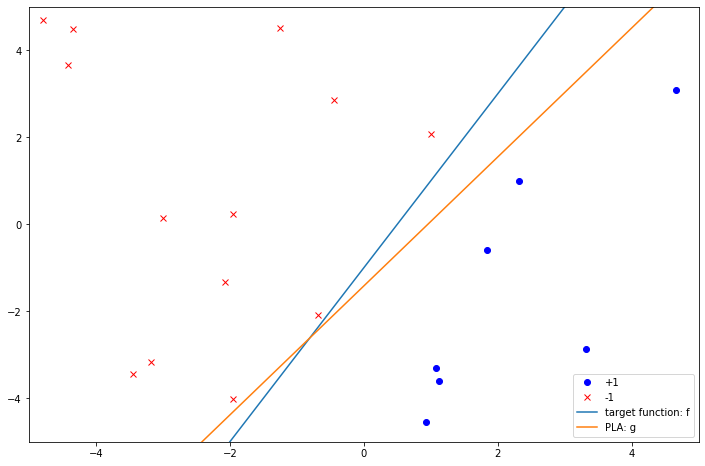
可以看到只经过5步PLA算法就收敛了，主要原因是这里的样本点本身比较少并且权重 $\mathbf{w}$ 的初始值 $\mathbf{0}$ 已经能将大部分点分开了。我们把这根线画到图上：

fig, ax = plt.subplots(1, 1, figsize=(12, 8))

ax.plot(X[y==1][:, 0], X[y==1][:, 1], color='blue', marker='o', linestyle='None', label='+1')
ax.plot(X[y==-1][:, 0], X[y==-1][:, 1], color='red', marker='x', linestyle='None', label='-1')

xs = np.arange(-5, 5, 0.1) # Generate plot data

ax.plot(xs, [-(w[0] + w[1] * x)/w[2] for x in xs], label='target function: f')
ax.plot(xs, [-(w_pla[0] + w_pla[1] * x)/w_pla[2] for x in xs], label='PLA: g')
ax.set_xlim(left=-5, right=5)
ax.set_ylim(bottom=-5, top=5)
ax.legend();

最后我们试着和sklearn中的PLA比较一下结果。

from sklearn.linear_model import Perceptron

clf = Perceptron(tol=1e-3)
clf.fit(X, y)

clf.score(X, y)  # Returns the mean accuracy on the given test data and labels.
                 # Here 1.0 means there is no error on the training set 

输出结果为：

1.0

这里返回的score值为1.0，说明感知机把我们的数据完全分开了，没有任何错误。

weight $\mathbf{w}$ 的值为 $(-3, 5.98783968, -1.78432935)^T$ .

clf.intercept_, clf.coef_

(array([-3.]), array([[ 5.98783968, -1.78432935]]))

我们把sklearn得到的线也画出来：

# Combine the intercept and coefficients 
w_skl = np.r_[clf.intercept_, clf.coef_.flatten()]

# Add the PLA result from sklearn
fig, ax = plt.subplots(1, 1, figsize=(12, 8))
ax.plot(X[y==1][:, 0], X[y==1][:, 1], color='blue', marker='o', linestyle='None', label='+1')
ax.plot(X[y==-1][:, 0], X[y==-1][:, 1], color='red', marker='x', linestyle='None', label='-1')

xs = np.arange(-5, 5, 0.1)

ax.plot(xs, [-(w[0] + w[1] * x)/w[2] for x in xs], label='target function: f')
ax.plot(xs, [-(w_pla[0] + w_pla[1] * x)/w_pla[2] for x in xs], label='PLA: g')
ax.plot(xs, [-(w_skl[0] + w_skl[1] * x)/w_skl[2] for x in xs], label='PLA from sklearn')

ax.set_xlim(left=-5, right=5)
ax.set_ylim(bottom=-5, top=5)
ax.legend();

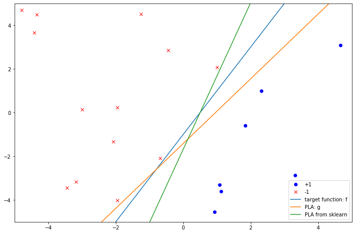
可以看到，不管是我们自己写的PLA，还是利用sklearn得到的感知机，都能完美地分割这组数据，但是它们又都不是目标函数本身。

针对有噪音数据：Pocket算法

上面生成的模拟数据是不带噪音的，而如果我们考虑噪音的影响，也就是说$f$得到$y$后又有一定概率$y$的符号会发生改变，那这时该怎么找函数$g$呢？

我们先看看带有噪音的数据是怎么样的（假设 $y$ 的符号翻转概率为$p=0.2$）。

def generateXY_with_noise(N, d, w, p):
    """
    Generate a random sample X of size N from a d-dimensional uniform distribution: [-5, 5]^d.
    Label each point by the target linear function described by weight vector w first 
    and then flip the result with probability p.
    
    Args:
        N: int, sample size
        d: int, number of features
        w: ndarray of shape = [d + 1, ], weight of the target linear function including bias w0
        p: float, the probablity of y that will flip
        
   Returns:
        X: ndarray of shape = [N, d], feature matrix
        y: ndarray of shape = [N, ], labels        
    """
    X = np.random.uniform(-5, 5, (N, d))
    X_ones = np.c_[np.ones((N, 1)), X]
    
    # Label each point by target function
    y = 2 * (X_ones @ w > 0) - 1  # y = +1 or -1
    
    # Flip the label y with probability p
    for i in range(N):
        rand_num = np.random.rand()
        if rand_num < p:
            y[i] = -y[i]
            
    return X, y

p = 0.2 # Probability that y will flip

# Set a random seed to get a persistent answer
np.random.seed(42)

X_noisy, y_noisy = generateXY_with_noise(N, d, w, p)

fig, ax = plt.subplots(1, 1, figsize=(12, 8))
ax.plot(X_noisy[y_noisy==1][:, 0], X_noisy[y_noisy==1][:, 1], color='blue', marker='o', linestyle='None', label='+1')
ax.plot(X_noisy[y_noisy==-1][:, 0], X_noisy[y_noisy==-1][:, 1], color='red', marker='x', linestyle='None', label='-1'); 

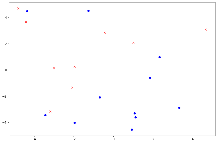
可以看到这个时候的数据不是线性可分的，因此PLA不收敛。那可不可以修改一下PLA得到一个“还不错”的 $g$ 呢？这就要提到Pocket算法了。

Pocket算法是一种贪心算法，它比普通的PLA的多了一个变量和一个步骤：

一个变量：用来记录手头上已有的最好的权重 $\mathbf{w}_{\text{pocket}}$ ；
一个步骤：权重每次更新后需要计算新的错误率并和已有的进行比较，如果新的错误率更低，就用这个新的权重替代已有的 $\mathbf{w}_{\text{pocket}}$ .

正是因为多出来的这一步，使得Pocket算法在速度上会比普通的PLA慢一些。下面是Pocket算法的实现：

def PLA_pocket(X, y, num_update=50):
    """
    Modified PLA algorithm by keeping best weights in pocket.
    
    Args:
        X: ndarray of shape = [n, d], feature matrix
        y: ndarray of shape = [n, ], labels
        num_update: int, default=50, number of updates for w_pocket to run on the data set
    
    Returns:
        w_pocket: ndarray of shape = [d + 1, ], best weights including bias w0
    """
    
    n, d = X.shape
    # Add a column of ones as first column
    X = np.c_[np.ones((n, 1)), X]
    
    # Initialize w to 0 and add an extra zero for w0
    w = np.zeros(d + 1)
    w_pocket = np.zeros(d + 1)
    
    smallest_error_rate = 1.0
    update_cnt = 0
    t = 0
    correct_num = 0
    
    while update_cnt < num_update and correct_num < n:
        x_t, y_t = X[t], y[t]
        if sign(w.T @ x_t) == y_t:
            correct_num += 1
        else:
            w += y_t * x_t
            update_cnt += 1
            correct_num = 0
            current_error_rate = error_rate(X, y, w)
            if current_error_rate < smallest_error_rate:
                w_pocket = w.copy()  #### NOTE: DO NOT write w_pocket=w directly, otherwise, w_pocket and w will point to the same object
                smallest_error_rate = current_error_rate
        if t == n - 1:
            t = 0
        else:
            t += 1   
            
    return w_pocket

################ Helper functions ################

# Vectorized version of sign function
sign_vec = np.vectorize(sign)


def error_rate(X, y, w):
    """
    Calculate the current error rate with the given weights w and examples (X, y).
    
    Returns:
        err: float, error rate 
    Argss
        X: ndarray of shape = [n, d + 1], feature matrix including a column of ones as first column
        y: ndarray of shape = [n, ], labels
        w: ndarray of shape = [d + 1, ], current weight
    """
    
    n = y.shape[0]
    err = np.sum(sign_vec(X @ w) != y) / n
    
    return err

将Pocket算法应用到带有噪音的数据上后：

w_pocket = PLA_pocket(X_noisy, y_noisy, num_update=100)
w_pocket

输出结果为：

array([ 2.        ,  1.80158115, -3.38519667])

错误率为：

error_rate(np.c_[np.ones((N, 1)), X_noisy], y_noisy, w_pocket)

0.2

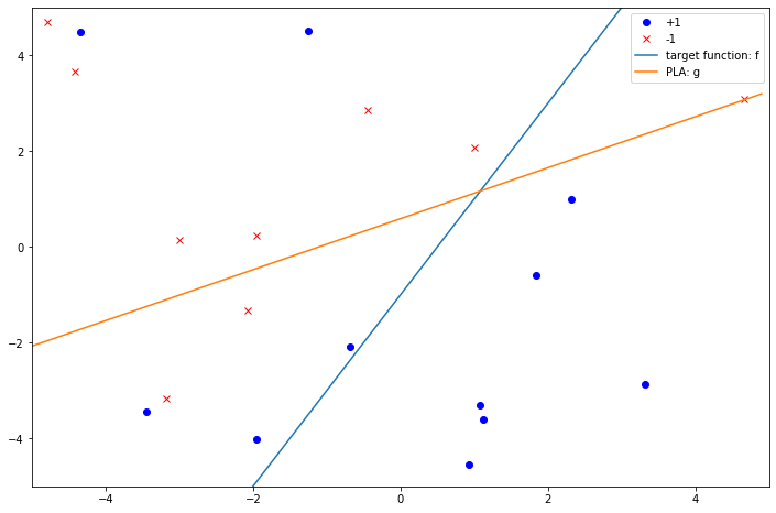
可以看到错误率为0.2，也就是20个点中有4个点错分了。考虑到$y$的符号翻转概率为0.2，因此20个点中平均会有4个点受到噪音的干扰。从这一点上来说，利用Pocket算法所获得的简单线性分类器，它在非线性可分的数据集上出错的平均个数也应该在4个左右，这和实际结果也是相符的。

将这个新的线性分类器作图如下：

fig, ax = plt.subplots(1, 1, figsize=(12, 8))

ax.plot(X_noisy[y_noisy==1][:, 0], X_noisy[y_noisy==1][:, 1], color='blue', marker='o', linestyle='None', label='+1')
ax.plot(X_noisy[y_noisy==-1][:, 0], X_noisy[y_noisy==-1][:, 1], color='red', marker='x', linestyle='None', label='-1')

xs = np.arange(-5, 5, 0.1) # Generate plot data

ax.plot(xs, [-(w[0] + w[1] * x)/w[2] for x in xs], label='target function: f')
ax.plot(xs, [-(w_pocket[0] + w_pocket[1] * x)/w_pocket[2] for x in xs], label='PLA: g')
ax.set_xlim(left=-5, right=5)
ax.set_ylim(bottom=-5, top=5)

ax.legend();

为了凸显出分类边界（也就是$g$），我们加入背景色（实际上是利用$g$对整个二维平面进行分类，得到密密麻麻的点）：用浅蓝色代表+1的区域，粉色代表-1的区域，结果如下：

x1_np = np.linspace(-5, 5, 100)
x2_np = np.linspace(-5, 5, 100)

blue_range = []
red_range = []

g = lambda x: sign(w_pocket @ x)

for i in range(len(x1_np)):
    for j in range(len(x2_np)):
        x = [x1_np[i], x2_np[j]]
        x_ext = np.r_[1, x]
        if g(x_ext) > 0:
            blue_range.append(x)
        else:
            red_range.append(x)
            
blue_range_np = np.array(blue_range)
red_range_np = np.array(red_range)

fig, ax = plt.subplots(1, 1, figsize=(12, 8))

ax.plot(X_noisy[y_noisy==1][:, 0], X_noisy[y_noisy==1][:, 1], color='blue', marker='o', markersize=8, linestyle='None', label='+1')
ax.plot(X_noisy[y_noisy==-1][:, 0], X_noisy[y_noisy==-1][:, 1], color='red', marker='x', markersize=8, linestyle='None', label='-1')

ax.plot(red_range_np[:, 0], red_range_np[:, 1], color='pink', marker='o', linestyle='None', alpha=0.2)
ax.plot(blue_range_np[:, 0], blue_range_np[:, 1], color='skyblue', marker='o', linestyle='None', alpha=0.2)

xs = np.arange(-5, 5, 0.1) 
# ax.plot(xs, [-(w[0] + w[1] * x)/w[2] for x in xs], label='target function: f')
ax.plot(xs, [-(w_pocket[0] + w_pocket[1] * x)/w_pocket[2] for x in xs], color='orange', label='PLA decision boundary')

ax.set_xlim(left=-5, right=5)
ax.set_ylim(bottom=-5, top=5)
ax.legend();

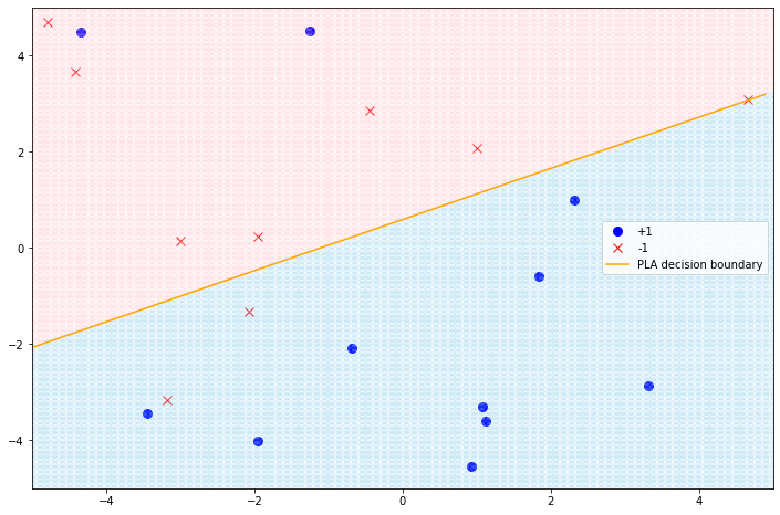
加上“背景色”后，我们就可以清楚地看到分类边界和错分点了。

参考文献

Abu-Mostafa, Y. S., Magdon-Ismail, M., & Lin, H. (2012). Learning from data: a short course. [United States]: AMLBook.com.