Machine Learning Foundations Homework 1

Website of Machine Learning Foundations by Hsuan-Tien Lin: https://www.csie.ntu.edu.tw/~htlin/mooc/.

Question 1

Which of the following problems are best suited for machine learning?

(i) Classifying numbers into primes and non-primes

(ii) Detecting potential fraud in credit card charges

(iii) Determining the time it would take a falling object to hit the ground

(iv) Determining the optimal cycle for traffic lights in a busy intersection

(v) Determining the age at which a particular medical test is recommended

Ans: (ii), (iv), (v)

Explanation

(i): False. Prime number has a programmable definition;

(iii): False. The underlying pattern is known by the physical equation $h=\frac{1}{2}g t^2$.

---

For Question 2-5, identify the best type of learning that can be used to solve each task below.

Question 2

Play chess better by practicing different strategies and receive outcomes as feedback

Ans: reinforcement learning

Explanation

We can make a reward or punishment to a single move. The machine can learn from these positive or negative feedbacks. So this is a type of reinforcement learning.

Question 3

Categorize books into groups without given topics

Ans: unsupervised learning

Explanation

We are not given labels at advance and need to let the machine classify books automatically. So this is a type of unsupervised learning.

Question 4

Recognize whether there is a face in the picture by a thousand face pictures and ten thousand non-face pictures.

Ans: supervised learning

Explanation

We are given the input and output labels together. So this is a type of a supervised learning.

Question 5

Selectively schedule experiments on mice to quickly evaluate the potential of cancer medicines.

Ans: active learning

Explanation

We want to know the potential of one cancer medicine, so we perform appropriate experiments to get the answer. This is like a “question-asking” procress and hence is a type of an active learning.

---

Question 6-8 are about Off-Training-Set error.

Let $\mathcal{X} = \{\mathbf{x}_1, \mathbf{x}_2, \cdots, \mathbf{x}_N, \mathbf{x}_{N+1}, \cdots, \mathbf{x}_{N+L}\}$ and $\mathcal{Y} = {-1, 1}$ (binary classfication). Here the set of training examples is $\mathcal{D} = \{(\mathbf{x}_n, y_n)\}_{n=1}^{N}$, where $y_n \in \mathcal{Y}$, and the set of test inputs is $\{\mathbf{x}_{N+\ell}\}_{\ell=1}^L$. The off-Training-Set error (OTS) with respect to an underlying target $f$ and a hypothesis $g$ is

$$E_{O T S}(g, f)=\frac{1}{L} \sum_{\ell=1}^{L}\left[g\left(\mathbf{x}_{N +\ell}\right) \neq f\left(\mathbf{x}_{N + \ell}\right)\right].$$

Question 6

Consider $f(\mathbf{x}) = +1$ for all $\mathbf{x}$ and,

$$g(\mathbf{x})=\left\{\begin{array}{lr} {+1,} & {\text { for } \mathbf{x}=\mathbf{x}_{k} \text { and } k \text { is odd and } 1 \leq k \leq N+L} \\ {-1,} & {\text { otherwise. }} \end{array}\right.$$

What is $E_{O T S}(g, f)$ ?

Ans: $\frac{1}{L} (\left\lfloor\frac{N+L}{2}\right\rfloor -\left\lfloor\frac{N}{2}\right\rfloor)$

Explanation

The question is equivalent to count the even numbers between $N+1$ and $N+L$.

For example, if $N = 101$ and $L=19$, then training examples are from $1$ to $101$ and test examples are from $102$ to $120$. So there are 10 even numbers bewteen $102$ and $120$.

Now, calculate $\frac{N+L}{2} = 60$ and $\frac{N}{2}=50.5$. Thus, $10 = \left\lfloor\frac{N+L}{2}\right\rfloor -\left\lfloor\frac{N}{2}\right\rfloor$.

By considering the 4 cases for the combination of $N$ (even/odd) and $L$ (even/odd), we can get the answer.

Question 7

We say that a target function $f$ can “generate” $\mathcal{D}$ in a noiseless setting if $f(\mathbf{x}_n) = y_n$ for all $(\mathbf{x}_n, y_n) \in \mathcal{D}$.

For all possible $f: \mathcal{X} \rightarrow \mathcal{Y}$, how many of them can generate $\mathcal{D}$ in a noiseless setting?

Note that we call two functions $f_1$ and $f_2$ the same if $f_1(\mathbf{x}) = f_2(\mathbf{x})$ for all $\mathbf{x} \in \mathcal{X}$.

Ans: $2^{L}$

Explanation

For a function $f$ to generate $\mathcal{D}$ in a noiseless setting, it must fit all the training data. So the only choice that such two functions can differ is on the test set. Since the size of the test set is $L$ and each label $y$ can only take two values, the total number of possible such functions is $2^L$.

Question 8

A deterministic algorithm $\mathcal{A}$ is defined as a procedure that takes $\mathcal{D}$ as an input, and outputs a hypothesis $g$. For any two deterministic algorithms $\mathcal{A}_1$ and $\mathcal{A}_2$, if all those $f$ that can “generate” $\mathcal{D}$ in a noiseless setting are equally likely in probability. Then which of the follow choices is correct?

(i) For any given $f$ that “generates” $\mathcal{D}$, $\left\{E_{O T S}\left(\mathcal{A}_{1}(\mathcal{D}), f\right)\right\}=\left\{E_{O T S}\left(\mathcal{A}_{2}(\mathcal{D}), f\right)\right\}$

(ii) For any given $f’$ that does not “generates” $\mathcal{D}$, $\left\{E_{O T S}\left(\mathcal{A}_{1}(\mathcal{D}), f^{\prime}\right)\right\}=\left\{E_{O T S}\left(\mathcal{A}_{2}(\mathcal{D}), f^{\prime}\right)\right\}$

(iii) $\mathbb{E}_{f}\left\{\operatorname{E}_{O T S}\left(\mathcal{A}_{1}(\mathcal{D}), f\right)\right\}=\mathbb{E}_{f}\left\{E_{O T S}\left(\mathcal{A}_{2}(\mathcal{D}), f\right)\right\}$

(iv) $\mathbb{E}_{f}\left\{\operatorname{E}_{O T S}\left(\mathcal{A}_{1}(\mathcal{D}), f\right)\right\}=\mathbb{E}_{f}\left\{E_{O T S}(f, f)\right\}$

(v) none of the other choices

Ans: (iii)

Explanation

(i) and (ii): Two different algorithms will produce two different hypothises, so the result of the error on the test set may not be the same regardless $f$ “gerneates” $\mathcal{D}$ or not.

(iv): $E_{O T S}(f, f)$ equals 0 and hence the RHS is 0, however, the LHS is not.

Now, we need to prove that $\mathbb{E}_{f}\left\{\operatorname{E}_{O T S}(\mathcal{A}(\mathcal{D}), f)\right\}=\text { constant },$

regardless of $\mathcal{A}$.

Proof: For a given hypothesis $g$ and an integer $k$ between $0$ and $L$, we claim that there are ${L}\choose{k}$ of those $f$ in Question 7 that satisfy $E_{O T S}(g, f) = \frac{k}{L}$.

Proof of the claim:

Since

$$E_{O T S}(g, f) = \frac{1}{L}\sum_{\ell=1}^{L}\left[g\left(\mathbf{x}_{N +\ell}\right) \neq f\left(\mathbf{x}_{N + \ell}\right)\right]=\frac{k}{L},$$

we know $f$ and $g$ differ on $k$ of those $\mathbf{x}_{N+\ell}$’s. Hence, the possible number of $f$ is ${L}\choose{k}$.

Now, we want to calculuate the expectation of off training-set error $\mathbb{E}_{f}\left\{E_{O T S}\left(g, f\right)\right\}$ for a fixed hypothesis $g$ and we will see it is a constant.

Since we are assuming all of $f$ are equally likely in probability, $E_{O T S}\left(g, f\right)$ is a discrete random variable (remember $g$ is fixed now) which has a distribution like:

value	$0$	$\frac{1}{L}$	$\frac{2}{L}$	$\cdots$	$\frac{k}{L}$	$\cdots$	$\frac{L-1}{L}$	$1$
probability	$\frac{L\choose 0}{2^L}$	$\frac{L\choose 1}{2^L}$	$\frac{L\choose 2}{2^L}$	$\cdots$	$\frac{L\choose k}{2^L}$	$\cdots$	$\frac{L\choose L-1}{2^L}$	$\frac{L\choose L}{2^L}$

Therefore,

$$\begin{aligned} \mathbb{E}_{f}\left\{E_{\text {OTS }}(g, f)\right\} &=\sum_{k=0}^{L} \frac{L \choose k}{2^{L}} \cdot \frac{k}{L} \\ &=\sum_{k=1}^{L} \frac{L-1 \choose k-1}{2^L} \cdot L \cdot \frac{1}{L} \\ &=\frac{1}{2^L} \sum_{k=1}^{L} {L-1 \choose k-1} \\ &=\frac{2^{L-1}}{2^{L}} \\ &=\frac{1}{2}.\end{aligned}$$

Here we use the equality $k {L \choose k} = {L-1 \choose k-1 }L$.

Finally, we proceed to prove the desired result: $\mathbb{E}_{f}\left\{\operatorname{E}_{O T S}(\mathcal{A}(\mathcal{D}), f)\right\}=\text { constant },$

regardless of $\mathcal{A}$.

However, we have just proved that $\mathbb{E}_{f}\left\{\operatorname{E}_{O T S}(g, f)\right\}$ is a constant for any hypothesis $g$ and thus, the result holds.

---

For Question 9-12, consider the bin model introduced in class.

Question 9

Consider a bin with infinitely man marbles, and let $\mu$ be the fraction of orange marbles in the bin, and $\nu$ is the fraction of orange marbles in a sample of 10 marbles.

If $\mu=0.5$, what is the probability of $\nu=\mu$ ?

Ans: 0.2461

Explanation

Method 1

def choose(n, k):
    """
    Returns the combination number n choose k.
    """
    from math import factorial
    return int(factorial(n) / (factorial(n-k) * factorial(k)))

n = 10
mu = 0.5
k = n * mu
prob_nu_eq_mu = choose(n, k) * (mu ** k) * (1 - mu) ** (n - k)
print(prob_nu_eq_mu)

0.246093

Method 2

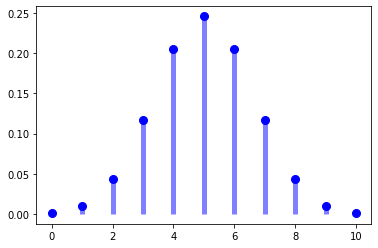
Let $X$ be the number of orange marbles in the sample. Since the bin is assumed to have infinitely many marbles, we can treate $X$ as a sum of i.i.d Bernouli random variables $\text{Bernouli}(p)$ with success probability $p=\mu$. Then $X$ has a binomial distribution $\text{binomial}(10, 0.5)$.

In the meanwhile,

$$\nu = 0.5 \iff X=5,$$

hence

$$P(\nu=0.5) = P(X=5) = {10 \choose 5} \left(\frac{1}{2}\right)^5 \left(1-\frac{1}{2}\right)^{10-5} \approx 0.2461.$$

Here is what the distribution of $X$ looks like.

from scipy.stats import binom
import numpy as np
import matplotlib.pyplot as plt

n, p = 10, 0.5
xs = list(range(0, 11))
probs = [binom.pmf(x, n, p) for x in xs]

fig, ax = plt.subplots(1, 1)
ax.plot(xs, probs, 'bo', ms=8, label='binom pmf')
ax.vlines(xs, 0, probs, colors='b', lw=5, alpha=0.5);

rv = binom(n, p)
print(rv.pmf(5))   # Verify P(X=5)=0.2461

0.24609375000000025

Question 10

If $\mu = 0.9$, what is the probability of $\nu=\mu$ ?

Ans: $P(\nu=0.9)= P(X=9)=0.3874$

mu = 0.9
k = n * mu
prob_nu_eq_mu = choose(n, k) * (mu ** k) * (1 - mu) ** (n - k)
print(prob_nu_eq_mu)

0.38742048900000003

Verify the result using binom function:

p = 0.9
rv = binom(n, p)
print(rv.pmf(9))  # Verify P(X=9)

0.38742048900000037

Question 11

If $\mu = 0.9$, what is the probability of $\nu \le 0.1$ ?

Ans: $P(\nu \le 0.1) = P(X \le 1)=9.0999\times 10^{-9}$

k = 0
prob_x_eq_0 = choose(n, k) * (mu ** k) * (1 - mu) ** (n - k)
k = 1
prob_x_eq_1 = choose(n, k) * (mu ** k) * (1 - mu) ** (n - k)
prob_nu_le_01 = prob_x_eq_0 + prob_x_eq_1
print(prob_nu_le_01)

9.09999999999998e-09

Verify the result:

print(binom.pmf(0, n, p) + binom.pmf(1, n, p))

9.099999999999995e-09

Question 12

If $\mu=0.9$, what is the bound given by Hoeffding’s inequality for the probability $\nu \le 0.1$ ?

Ans: $5.52\times 10^{-6}$

Explanation

Recall Hoeffding’s inequality:

$$\mathbb{P}(|\nu-\mu|>\epsilon) \leq 2 \exp \left(-2 \epsilon^{2} N\right).$$

Substitute our data, we can get

$$\begin{align} \mathbb{P}\left(\nu \le 0.1\right) &= \mathbb{P}\left(\nu - 0.9 \le 0.1 - 0.9\right) \\ &\le \mathbb{P}\left(\left| \nu - 0.9 \right| \ge 0.8 \right). \end{align}$$

Hence, we have $\epsilon=0.8$ here and the answer follows.

def hoeffding_ineq(epsilon, N):
    """
    Returns the bound by hoeffding's inequality.
    """
    from numpy import exp
    return 2 * exp(-2 * epsilon ** 2 * N)

print(hoeffding_ineq(0.8, 10))

5.521545144074388e-06

---

Question 13-14 illustate what happens with multiple bins using dice to indicate 6 bins. Please note that the dice is not meant to be thrown for random experiments in this problem. They are just used to bind the six faces together. The probability below only refers to drawing from the bag.

Question 13

Consider four kinds of dice in a bag, with the same (super large) quantity for each kind.

A: all even numbers are colored orange, all odd numbers are colored green

B: all even numbers are colored green, all odd numbers are colored orange

C: all small(1-3) are colored orange, all large numbers(4-6) are colored green

D: all small(1-3) are colored green, all large numbers(4-6) are colored orange

If we pick 5 dice from the bag, what is the probability that we get five orange 1’s?

Ans: $\frac{1}{32}$

Explanation

Notice that only dice B and C have orange 1, so the total probability of getting five orange 1’s is $(\frac{1}{2})^5=\frac{1}{32}$.

Question 14

If we pick 5 dice from the bag, what is the probability that we get “some number” that is purely orange?

Ans: $\frac{31}{256}$

Explanation

Let $X_i$ be the total number of orange faces for number $i$ in 5 dice, $i=1, \cdots, 6$. We want to calculate the probability that at least one of $X_i$ is 5, i.e.,

$$\mathbb{P} \left(\{X_1 = 5\} \cup \{X_2 = 5\} \cup \cdots \cup \{X_6 = 5\}\right).$$

Notice that number 1 and number 3 always take on the same color and so do 4 and 6. Meanwhile, we cannot see number 2 and 5 having the same color no matter what kind of dice we get, neither do 1 and 4.

Thus, we can simplify the above probability a bit by removing $X_3$ and $X_6$:

$$\mathbb{P} \left(\{X_1 = 5\} \cup \{X_2 = 5\} \cup \{X_4 = 5\} \cup \{X_5 = 5\}\right).$$

We can use inclusion-exclusion principle to calculate the above probability. So we need probability for individual event, for intersection of two, three, and four events, respectively.

The probability of a single event is straightfoward: $\mathbb{P}({X_i=5})=(\frac{1}{2})^5=\frac{1}{32}$.

As for intersection of two events:

• ${X_1=5}$ and ${X_2=5}$ can both occur if and only if all 5 dice are of type C;
• ${X_1=5}$ and ${X_4=5}$ cannot both occur at the same time because 1 and 4 cannot have the same color;
• ${X_1=5}$ and ${X_5=5}$ can both occur if and only if all 5 dice are of type B;
• ${X_2=5}$ and ${X_4=5}$ can both occur if and only if all 5 dice are of type A;
• ${X_2=5}$ and ${X_5=5}$ cannot both occur at the same time because 2 and 5 cannot have the same color;
• ${X_4=5}$ and ${X_5=5}$ can both occur if and only if all 5 dice are of type D.

The probability of each intersection is $(\frac{1}{4})^5=\frac{1}{1024}$.

As for intersection of three (or four), there are no three such events that can occur at the same time. Hence the probability is 0.

By inclusion-exclusion principle, $\mathbb{P} \left(\{X_1 = 5\} \cup \{X_2 = 5\} \cup \{X_4 = 5\} \cup \{X_5 = 5\}\right) = 4 \cdot \frac{1}{32} - 4 \cdot \frac{1}{1024} = \frac{31}{256}.$

---

For Question 15-20, you will play with PLA and pocket algorithm. First, we use an artificial data set to study PLA. The data set is in hw1_15_train.dat.

Question 15

Each line of the data set contains one $(\mathbf{x}_n, y_n)$ with $\mathbf{x}_n \in \mathbb{R}^4$. The first 4 numbers of the line contains the components of $\mathbf{x}_n$ orderly, the last number is $y_n$.

Please initialize your algorithm with $\mathbf{w}=0$ and take sign(0) as $-1$.

Implement a version of PLA by visiting examples in the naive cycle using the order of examples in the data set. Run the algorithm on the data set. What is the number of updates before the algorithm halts?

import pandas as pd

# Load data
data = pd.read_csv('hw1_15_train.dat', sep='\s+', header=None, names=['x1', 'x2', 'x3', 'x4', 'y'])

# Construct features and labels
y = data['y'].to_numpy()
X = data[['x1', 'x2', 'x3', 'x4']].to_numpy()

def PLA_cyclic(X, y):
    """
    PLA by visiting examples in the naive cycle using the order of examples in the data set (X, y).
    
    Args:
        X: numpy array(n, d), feature matrix
        y: numpy array(n, ), labels
    Returns:
        w         : numpy array(d+1, ), final weights including bias w0
        update_cnt: the total number of updates 
    """
    
    n, d = X.shape
    # Add a column of ones as first column
    X = np.c_[np.ones((n, 1)), X]
    
    # Initialize w to 0 and add an extra zero for w0
    w = np.zeros(d + 1)
        
    # Count the number of updates
    update_cnt = 0 
    
    is_finished = 0
    correct_num = 0
    t = 0

    while not is_finished:
        x_t, y_t = X[t], y[t]
        
        if sign(w.T @ x_t) == y_t:  # Correctly classify the current example
            correct_num += 1
        else:                       # Find a mistake
            w += y_t * x_t          # Correct the mistake
            update_cnt += 1         # Increment update count
            correct_num = 0         # Reset correct num to 0 to retest the new w
        if t == n - 1:              # Start the next cycle
            t = 0
        else:
            t += 1
        if correct_num == n:        # Have all examples classified correctly
            is_finished = 1
  
    return w, update_cnt

                
######## Some helper functions ########
def sign(x):
    return 1 if x > 0 else -1

w, t = PLA_cyclic(X, y)

print(w)

array([-3.       ,  3.0841436, -1.583081 ,  2.391305 ,  4.5287635])

print(t)

45

So the total number of updates before the algorithm halts is 45 times under my implementation of PLA with naive cycling.

Question 16

Implement a version of PLA by visiting examples in fixed, pre-determined random cycles throughout the algorithm. Run the algorithm on the data set.

Please repeat your experiment for 2000 times, each with a different random seed. What is the average number of updates before the algorithm halts?

def PLA_random(X, y):
    """
    PLA by visiting examples in a fixed, pre-determined random cycles.
    
    Note: it repeat experiment for 2000 times.
    seed.
    
    Args:
        X: numpy array(n, d), feature matrix
        y: numpy array(n, ), labels
    Returns:
        w         : numpy array(d+1, ), final weights including bias w0
        update_cnt: the average number of updates 
    """
    T = 2000
    t_list = []
    n = X.shape[0]
    indices = np.arange(n)
    
    for i in range(T):
        # Shuffle X and y together using random indices
        np.random.shuffle(indices)  
        X = X[indices]
        y = y[indices]
        w, t = PLA_cyclic(X, y)
        t_list.append(t)
        print(f"{i}th experiment: {t} updates!")
    return w, int(np.mean(t_list))
    

w, t = PLA_random(X, y)

print(w)

array([-3.        ,  2.30784   , -1.133837  ,  2.110653  ,  4.34285278])

print(t)

39

If we visit examples in fixed, pre-determined random cycles, then the average number of updates is 39.

Question 17

Implement a version of PLA by visiting examples in fixed, pre-determined random cycles throughout the algorithm, while changing the update rule to be

$$\mathbf{w}_{t+1} \leftarrow \mathbf{w}_{t}+\eta y_{n(t)} \mathbf{x}_{n(t)}$$

with $\eta=0.5$. Note that your PLA in the previous Question corresponds to $\eta=1$. Please repeat your experiment for 2000 times, each with a different random seed. What is the average number of updates before the algorithm halts?

def PLA_random_eta(X, y, eta=1.0):
    """
    PLA by visiting examples in a fixed, pre-determined random cycles
    and update the weight using the given learning rate eta with default
    value 1.0.

    Note: It repeat experiment for 2000 times.
    
    Args:
        X  : numpy array(n, d), feature matrix
        y  : numpy array(n, ), labels
        eta: double, learning rate
    Returns:
        w         : numpy array(d+1, ), final weights including bias w0
        update_cnt: the average number of updates 
    """
    T = 2000
    t_list = []
    n = X.shape[0]
    indices = np.arange(n)
    
    for i in range(T):
        # Shuffle X and y together using random indices
        np.random.shuffle(indices)  
        X = X[indices]
        y = y[indices]
        w, t = PLA_cyclic_eta(X, y, eta)
        t_list.append(t)
        print(f"{i}th experiment: {t} updates!")
    return w, int(np.mean(t_list))


def PLA_cyclic_eta(X, y, eta):
    """
    PLA by visiting examples in the naive cycle using the order of examples in the data set (X, y).
    
    Args:
        X: numpy array(n, d), feature matrix
        y: numpy array(n, ), labels
    Returns:
        w         : numpy array(d+1, ), final weights including bias w0
        update_cnt: the total number of updates 
    """
    
    n, d = X.shape
    # Add a column of ones as first column
    X = np.c_[np.ones((n, 1)), X]
    # Initialize w to 0 and add an extra zero for w0
    w = np.zeros(d + 1)
        
    # Count the number of updates
    update_cnt = 0 
    
    is_finished = 0
    correct_num = 0
    t = 0

    while not is_finished:
        x_t, y_t = X[t], y[t]
        
        if sign(w.T @ x_t) == y_t:  # Correctly classify the current example
            correct_num += 1
        else:                       # Find a mistake
            w += eta * y_t * x_t    # Correct the mistake
            update_cnt += 1         # Increment update count
            correct_num = 0         # Reset correct num to 0 to retest the new w
        if t == n - 1:              # Start the next cycle
            t = 0
        else:
            t += 1
        if correct_num == n:        # Have all examples classified correctly
            is_finished = 1
  
    return w, update_cnt

w, t = PLA_random_eta(X, y, eta=0.5)

print(w)

array([-2.        ,  1.567752  , -1.0663645 ,  1.8937115 ,  2.54472475])

print(t)

40

With learning rate $\eta=0.5$, the average number of updates is 40.

Question 18

Next, we play with the pocket algorithm. Modify your PLA in Question 16 to visit examples purely randomly, and then add the ‘pocket’ steps to the algorithm. We will use hw1_18_train.dat as the training data set $\mathcal{D}$ and hw1_18_test.dat as test set for verifying the g returned by your algorithm (see lecture 4 about verifying). The sets are of the same format as the previous one. Run the pocket algorithm with a total of 50 updates on $\mathcal{D}$, and verify the performance of $\mathbf{w}_{\text{POCKET}}$ using the test set. Please repeat your experiment for 2000 times, each with a different random seed. What is the average error rate on the test set?

# Load data
train_data = pd.read_csv('hw1_18_train.dat', sep='\s+', header=None, names=['x1', 'x2', 'x3', 'x4', 'y'])
test_data = pd.read_csv('hw1_18_test.dat', sep='\s+', header=None, names=['x1', 'x2', 'x3', 'x4', 'y'])

# Construct features and labels
y_train = train_data['y'].to_numpy()
X_train = train_data[['x1', 'x2', 'x3', 'x4']].to_numpy()

y_test = test_data['y'].to_numpy()
X_test = test_data[['x1', 'x2', 'x3', 'x4']].to_numpy()

def PLA_pocket(X, y, num_update=50):
    """
    Modified PLA algorithm by keeping best weights in pocket.
    
    Args:
        X         : numpy array(n, d), feature matrix
        y         : numpy array(n, ), labels
        num_update: int, number of updates of w_pocket to run on the data set
    
    Returns:
        w_pocket: numpy array(d + 1, ), best weights including bias w0
    """
    
    n, d = X.shape
    # Add a column of ones as first column
    X = np.c_[np.ones((n, 1)), X]
    
    # Initialize w to 0 and add an extra zero for w0
    w = np.zeros(d + 1)
    w_pocket = np.zeros(d + 1)
    
    smallest_error_rate = 1.0
    update_cnt = 0
    t = 0
    correct_num = 0
    
    while update_cnt < num_update and correct_num < n:
        x_t, y_t = X[t], y[t]
        if sign(w.T @ x_t) == y_t:
            correct_num += 1
        else:
            w += y_t * x_t
            update_cnt += 1
            correct_num = 0
            current_error_rate = error_rate(X, y, w)
            if current_error_rate < smallest_error_rate:
                w_pocket = w.copy()  #### NOTE: DO NOT write w_pocket=w directly, otherwise, w_pocket and w will point to the object
                smallest_error_rate = current_error_rate
        if t == n - 1:
            t = 0
        else:
            t += 1   
            
    return w_pocket


################ Helper functions ################

# Vectorized version of sign function
sign_vec = np.vectorize(sign)


def error_rate(X, y, w):
    """
    Calculate the current error rate with the given weights w and examples (X, y).
    
    Returns:
        err: double, error rate 
    Argss
        X: numpy array(n, d + 1), feature matrix including a column of ones as first column
        y: numpy array(n, ), labels
        w: numpy array(d + 1, ), current weight
    """
    
    n = y.shape[0]
    err = np.sum(sign_vec(X @ w) != y) / n
    
    return err
    

Note: the correct step w_pocket = w.copy() instead of w_pocket = w is where I made a mistake when implementing the algorithm and I took a lot of time before identifying the bug.

def PLA_pocket_test_random(X_train, y_train, X_test, y_test, num_updates=50):
    """
    Train PLA by pocket algorithm using trainning set and test on test set. 
    Repeat experiment for 2000 times and return average error rate.
    
    Note: we visit examples purely randomly
    
    Args:
        X_train    : numpy array(n, d), training feature matrix
        y_train    : numpy array(n, ), training labels
        X_test     : numpy array(m, d), test feature matrix
        y_test     : numpy array(m, ), test labels
        num_updates: int, number of updates of pocket weights to run on the data set
    Returns:
        avg_error: the average of error rate
    """

    n = X_test.shape[0]
    X_test = np.c_[np.ones((n, 1)), X_test]

    T = 2000
    indices = np.arange(n) 
    total_error = 0.0

    for i in range(T):
        np.random.shuffle(indices)  
        X_train = X_train[indices]
        y_train = y_train[indices]
        w = PLA_pocket(X_train, y_train, num_updates)
        error = error_rate(X_test, y_test, w)
#         print("error on test set:", error)
        total_error += error
        
    avg_error = total_error / T
    
    return avg_error

print(PLA_pocket_test_random(X_train, y_train, X_test, y_test, 50))

0.13146899999999967

The average error rate on the test set is about 0.13 on my computer.

Question 19

Modify your algorithm in Question 18 to return $\mathbf{w}_{50}$ (the PLA vector after 50 updates) instead of $\hat{\mathbf{w}}$ (the pocket vector) after 50 updates. Run the modified algorithm on $\mathcal{D}$, and verify the performance using the test set. Please repeat your experiment for 2000 times, each with a different random seed. What is the average error rate on the test set?

def PLA_fixed_updates_test_random(X_train, y_train, X_test, y_test, num_update):
    """
    Train PLA by pocket algorithm using trainning set and test on test set. 
    Repeat experiment for 2000 times and return average error rate.
    
    Note: we visit examples purely randomly
    
    Args:
        X_train   : numpy array(n, d), training feature matrix
        y_train   : numpy array(n, ), training labels
        X_test    : numpy array(m, d), test feature matrix
        y_test    : numpy array(m, ), test labels
        num_update: int, number of updates of weights to run on the data set
    Returns:
        avg_error: the average of error rate
    """

    n = X_test.shape[0]
    X_test = np.c_[np.ones((n, 1)), X_test]

    T = 2000
    indices = np.arange(n) 
    total_error = 0.0

    for i in range(T):
        np.random.shuffle(indices)  
        X_train = X_train[indices]
        y_train = y_train[indices]
        w = PLA_fixed_updates(X_train, y_train, num_update)
        error = error_rate(X_test, y_test, w)
#         print("error on test set:", error)
        total_error += error
        

    avg_error = total_error / T
    return avg_error


def PLA_fixed_updates(X, y, num_update=50):
    """
    Returns the weights after the required number of updates.
    
    Args:
        X         : numpy array(n, d), feature matrix
        y         : numpy array(n, ), labels
        num_update: int, number of updates of weights to run on the data set
    
    Returns:
        w: numpy array(d + 1, ), weights(including bias w0) after the required number of updates
    """
    
    n, d = X.shape
    # Add a column of ones as first column
    X = np.c_[np.ones((n, 1)), X]
    
    # Initialize w to 0 and add an extra zero for w0
    w = np.zeros(d + 1)
    
    update_cnt = 0
    t = 0
    correct_num = 0
    
    while update_cnt < num_update and correct_num < n:
        x_t, y_t = X[t], y[t]
        if sign(w.T @ x_t) == y_t:
            correct_num += 1
        else:
            w += y_t * x_t
            update_cnt += 1
            correct_num = 0
        if t == n - 1:
            t = 0
        else:
            t += 1   
            
    return w

print(PLA_fixed_updates_test_random(X_train, y_train, X_test, y_test, 50))

0.36959099999999995

The average error on the test set is about 0.37.

Question 20

Modify your algorithm in Question 18 to run for 100 updates instead of 50, and verify the performance of $\mathbf{w}_{\text{POCKET}}$ using the test set. Please repeat your experiment for 2000 times, each with a different random seed. What is the average error rate on the test set?

print(PLA_pocket_test_random(X_train, y_train, X_test, y_test, 100))

0.11417099999999998

The average error rate on the test set is about 0.11.